Train a model
FYI, you can open this documentation as a Google Colab notebook to follow along interactively
graph-pes-train provides a unified interface to train any GraphPESModel, including those packaged within graph_pes.models, custom ones defined by you, and any of the wrapper interfaces that graph-pes provides to other machine learning frameworks.
For more information on the graph-pes-train command, and the plethora of options available for specification in your config.yaml see the CLI reference.
Below, we train a lightweight NequIP model on the C-GAP-17 dataset.
Installation
[1]:
!pip install graph-pes
Successfully installed graph-pes-0.0.34
We should now have access to the graph-pes-train command. We can check this by running:
[14]:
!graph-pes-train -h
usage: graph-pes-train [-h] [args ...]

Train a GraphPES model using PyTorch Lightning.

positional arguments:
  args        Config files and command line specifications. Config files
              should be YAML (.yaml/.yml) files. Command line specifications
              should be in the form my/nested/key=value. Final config is built
              up from these items in a left to right manner, with later items
              taking precedence over earlier ones in the case of conflicts.

optional arguments:
  -h, --help  show this help message and exit

Copyright 2023-25, John Gardner
Data definition
When training a model, we typically want 3 sets of data (i.e. labelled atomic structures): a training set, a validation set, and a test set.
Below, we use load-atoms to download and split the C-GAP-17 dataset into training, validation and test datasets, and write these to xyz files. (graph-pes supports other dataset formats too, including ase sqlite databases – see here for more details)
[15]:
import ase.io
from load_atoms import load_dataset

structures = load_dataset("C-GAP-17")
train, val, test = structures.random_split([0.8, 0.1, 0.1])

ase.io.write("train-cgap17.xyz", train)
ase.io.write("val-cgap17.xyz", val)
ase.io.write("test-cgap17.xyz", test)
We can visualise the kinds of structures we’re training on using load_atoms.view:
[16]:
from load_atoms import view

view(train[0], show_bonds=True)
[16]:
As you can see, each structure has an energy label:
[17]:
train[0].info["energy"]
[17]:
-5643.968171
… as well as a forces label (one for each atom in the structure):
[19]:
train[0].arrays["forces"].shape
[19]:
(36, 3)
These properties are stored in the files we have just created:
[20]:
!head train-cgap17.xyz
36
Lattice="6.439806 0.0 0.0 0.0 6.439806 0.0 0.0 0.0 8.586408" Properties=species:S:1:pos:R:3:forces:R:3 config_type=bulk_amo detailed_ct=iter4_2 split=train energy=-5643.968171 pbc="T T T"
C      -10.19681458       4.52108512       2.58260263       1.92054269       0.70905554       3.23398419
C        8.88245018      10.54923296       9.85602863      -8.61008207       4.76824471      10.54597273
C      -12.37947091       3.12898582       0.00437048       0.40437923      -0.84438408       0.64039651
C      -15.36751513       3.67112089       7.46005158      -2.19558355      -5.72081017     -10.70417213
C        1.48348659       8.44603096      -5.40849254       2.13894508      -3.77202448       2.30942937
C        6.68203286       2.50162636     -11.97770429       0.95262647      -0.03136726      -0.79207429
C      -15.10503508       0.29261834       6.90345486      -2.22105290       2.34675963      -6.38519060
C       -4.49987240       0.25155170      -7.21023863       0.27927988       0.68979268       1.56306647
Configuration
Now that we’ve saved our labelled structures to suitable files, we’re ready to train a model.
To do this, we have specified the following in the quickstart-cgap17.yaml file:
the model architecture to instantiate and train, here NequIP. Note that we also include a FixedOffset component to account for the fact that the C-GAP-17 labels have an arbitrary offset.
the data to train on, here a random split of the C-GAP-17 dataset we just downloaded
the loss function to use, here a combination of a per-atom energy loss and a per-atom force loss
and various other training hyperparameters (e.g. the learning rate, batch size, etc.)
quickstart-cgap17.yaml
# define a radial cutoff to use throughout the config
CUTOFF: 3.7 # in Å

general:
    progress: logged

# train a lightweight NequIP model ...
model:
    offset:
        # note the "+" prefix syntax: refer to the
        # data2objects package for more details
        +FixedOffset: { C: -148.314002 }
    many-body:
        +NequIP:
            elements: [C]
            cutoff: =/CUTOFF # reference the radial cutoff defined above
            layers: 2
            features:
                channels: [16, 8, 4]
                l_max: 2
                use_odd_parity: true
            self_interaction: linear

# ... on structures from local files ...
data:
    train:
        path: train-cgap17.xyz
        n: 1280
        shuffle: false
    valid: val-cgap17.xyz
    test: test-cgap17.xyz

# ... on both energy and forces (weighted 1:1) ...
loss:
    - +PerAtomEnergyLoss()
    - +ForceRMSE()

# ... with the following settings ...
fitting:
    trainer_kwargs:
        max_epochs: 250
        accelerator: auto
        check_val_every_n_epoch: 5

    optimizer:
        name: AdamW
        lr: 0.01

    scheduler:
        name: ReduceLROnPlateau
        factor: 0.5
        patience: 10

    loader_kwargs:
        batch_size: 64

# ... and log to Weights & Biases
wandb:
    project: graph-pes-quickstart
You can download this config file using wget:
[4]:
%%bash

if [ ! -f quickstart-cgap17.yaml ]; then
    wget https://tinyurl.com/graph-pes-quickstart-cgap17 -O quickstart-cgap17.yaml
fi
Training
To train the model, we use the graph-pes-train command.
You can see the output of the original training run I ran in this Weights and Biases dashboard.
[12]:
!graph-pes-train quickstart-cgap17.yaml general/run_id=train-nequip
[graph-pes INFO]: Started `graph-pes-train` at 2025-04-11 11:21:47.393
[graph-pes INFO]: Successfully parsed config.
[graph-pes INFO]: Logging to graph-pes-results/train-nequip/rank-0.log
[graph-pes INFO]: ID for this training run: train-nequip
[graph-pes INFO]:
Output for this training run can be found at:
└─ graph-pes-results/train-nequip
├─ rank-0.log # find a verbose log here
├─ model.pt # the best model (according to valid/loss/total)
├─ lammps_model.pt # the best model deployed to LAMMPS
├─ train-config.yaml # the complete config used for this run
└─ summary.yaml # the summary of the training run
GPU available: True (cuda), used: True
TPU available: False, using: 0 TPU cores
HPU available: False, using: 0 HPUs
wandb: Using wandb-core as the SDK backend. Please refer to https://wandb.me/wandb-core for more information.
wandb: Currently logged in as: jla-gardner to https://api.wandb.ai. Use `wandb login --relogin` to force relogin
wandb: Tracking run with wandb version 0.19.9
wandb: Run data is saved locally in graph-pes-results/wandb/run-20250411_112150-train-nequip
wandb: Run `wandb offline` to turn off syncing.
wandb: Syncing run train-nequip
wandb: ⭐️ View project at https://wandb.ai/jla-gardner/graph-pes-quickstart
wandb: 🚀 View run at https://wandb.ai/jla-gardner/graph-pes-quickstart/runs/train-nequip
[graph-pes INFO]: Preparing data
[graph-pes INFO]: Setting up datasets
[graph-pes INFO]: Pre-fitting the model on 1,280 samples
[graph-pes INFO]:
Number of learnable params:
offset (FixedOffset): 0
many-body (NequIP) : 4,233
[graph-pes INFO]: Sanity checking the model...
[graph-pes INFO]: Starting fit...
LOCAL_RANK: 0 - CUDA_VISIBLE_DEVICES: [0]
/home/calcite/vld/jesu2890/graph-pes/.venv/lib/python3.9/site-packages/pytorch_lightning/trainer/connectors/data_connector.py:425: The 'val_dataloader' does not have many workers which may be a bottleneck. Consider increasing the value of the `num_workers` argument` to `num_workers=35` in the `DataLoader` to improve performance.
/home/calcite/vld/jesu2890/graph-pes/.venv/lib/python3.9/site-packages/pytorch_lightning/trainer/connectors/data_connector.py:425: The 'train_dataloader' does not have many workers which may be a bottleneck. Consider increasing the value of the `num_workers` argument` to `num_workers=35` in the `DataLoader` to improve performance.
/home/calcite/vld/jesu2890/graph-pes/.venv/lib/python3.9/site-packages/pytorch_lightning/loops/fit_loop.py:310: The number of training batches (20) is smaller than the logging interval Trainer(log_every_n_steps=50). Set a lower value for log_every_n_steps if you want to see logs for the training epoch.
valid/metrics valid/metrics valid/metrics valid/metrics valid/metrics valid/metrics timer/its_per_s timer/its_per_s
epoch time per_atom_energy_rmse per_atom_energy_mae energy_rmse energy_mae forces_rmse forces_mae train valid
5 8.7 0.62315 0.48031 35.21251 29.65179 1.39054 1.04576 21.27660 36.14532
10 17.3 0.25256 0.12514 8.46061 6.64184 1.06623 0.81321 21.27660 36.29926
15 25.8 0.30826 0.27898 20.66504 16.95788 0.97669 0.75126 21.27660 35.42593
20 34.1 0.26312 0.23339 17.40298 14.02269 0.94271 0.72719 21.27660 36.31066
25 42.7 0.13665 0.10314 8.13669 6.32626 0.91978 0.70968 21.27660 36.44294
30 51.2 0.16764 0.12787 9.88240 7.46267 0.90267 0.69606 21.73913 36.60828
35 59.3 0.16015 0.13001 10.08410 7.73408 0.89099 0.68656 21.27660 36.47427
40 67.8 0.16035 0.13706 10.79822 8.60235 0.87526 0.67691 21.27660 36.45434
45 76.4 0.11800 0.08278 6.48016 4.68341 0.86985 0.67295 21.27660 36.45434
50 84.9 0.09155 0.05939 4.56686 3.27326 0.86002 0.66365 20.83333 36.28899
55 93.4 0.13949 0.11225 8.63337 6.53863 0.85629 0.66144 20.40816 36.28900
60 101.5 0.10444 0.07786 6.25070 4.86074 0.84143 0.64941 20.83333 36.60828
65 110.0 0.11025 0.08216 6.76819 5.04506 0.84349 0.65043 21.27660 36.44294
70 118.2 0.12537 0.10013 7.94580 5.97333 0.83898 0.64568 21.27660 36.63748
75 126.4 0.08905 0.05865 4.85177 3.39582 0.83235 0.64291 20.83333 36.00164
80 135.0 0.08428 0.05420 4.29199 3.05238 0.81563 0.62996 20.83333 36.14532
85 143.6 0.08458 0.05217 4.20698 2.94109 0.83121 0.64083 20.83333 36.43267
90 151.8 0.15399 0.13354 10.28086 8.12393 0.80666 0.62302 20.40816 36.31066
95 160.0 0.08045 0.04999 4.00663 2.77370 0.80932 0.62424 20.00000 36.19618
100 168.6 0.14926 0.13008 10.68001 8.59175 0.80941 0.62616 20.83333 36.00164
105 176.8 0.17366 0.15842 12.33288 10.00910 0.81932 0.63167 20.83333 36.44294
110 185.0 0.12503 0.10650 8.62543 6.94882 0.79976 0.61861 20.83333 36.14532
115 193.1 0.11280 0.09268 7.43654 5.89931 0.79611 0.61464 21.73913 36.76162
120 201.3 0.10204 0.07421 6.05022 4.22249 0.79113 0.61078 20.40816 36.33059
125 209.5 0.08550 0.05395 4.18860 2.93031 0.79094 0.61093 20.83333 36.01091
130 218.1 0.09214 0.06968 5.29362 4.10699 0.80209 0.61774 20.83333 36.48453
135 226.3 0.09654 0.07404 6.03257 4.73452 0.78720 0.60859 20.40816 36.15672
140 234.5 0.13333 0.11478 8.86486 7.14934 0.79077 0.61130 21.73913 36.33059
145 242.7 0.10346 0.08377 6.58328 5.23925 0.78829 0.60864 21.73913 36.49593
150 250.9 0.08593 0.05443 4.48703 3.11985 0.78729 0.60804 21.73913 36.31066
155 259.4 0.07854 0.05421 4.18323 3.20169 0.78762 0.60745 21.27660 36.14532
160 268.0 0.13054 0.11253 8.83321 7.05205 0.78856 0.61020 21.27660 36.61795
165 276.1 0.13436 0.11566 9.05795 7.12900 0.78077 0.60236 21.27660 36.47427
170 284.3 0.10105 0.07397 6.03266 4.18178 0.78658 0.60791 20.83333 36.61795
175 292.5 0.09442 0.07199 6.01171 4.44474 0.78398 0.60551 21.73913 36.00164
180 300.7 0.08973 0.07091 5.71718 4.47134 0.77670 0.60024 21.27660 36.00164
185 308.8 0.16145 0.14754 11.38972 9.28238 0.77806 0.60138 21.27660 36.63961
190 317.0 0.07035 0.04360 3.59079 2.42807 0.78680 0.60764 20.83333 36.44294
195 325.5 0.11411 0.09597 7.54478 5.83939 0.77606 0.59926 20.83333 36.28899
200 333.7 0.07146 0.04575 3.67843 2.56994 0.78213 0.60312 20.83333 36.44294
205 342.2 0.10034 0.07853 6.16118 4.51715 0.77907 0.60105 20.83333 36.02117
210 350.4 0.09016 0.06550 5.56907 3.87992 0.77324 0.59818 21.27660 36.45434
215 358.6 0.06793 0.04424 3.41206 2.43981 0.77539 0.59888 21.27660 36.78329
220 367.1 0.22132 0.21056 16.07953 13.36178 0.80770 0.62159 20.83333 36.44294
225 375.3 0.07922 0.05494 4.71128 3.32506 0.77587 0.59897 20.00000 36.00164
230 383.5 0.06517 0.04025 3.21447 2.26121 0.77772 0.60106 20.40816 36.28900
235 392.0 0.07309 0.04843 4.15934 2.81432 0.77288 0.59675 21.73913 36.14532
240 400.1 0.07428 0.05531 4.23787 3.27787 0.77770 0.59988 21.27660 36.31066
245 408.3 0.12987 0.11495 8.94932 7.16290 0.77176 0.59641 20.40816 36.29926
250 416.5 0.07047 0.05124 3.92862 3.03030 0.77647 0.60081 20.83333 36.48453
`Trainer.fit` stopped: `max_epochs=250` reached.
[graph-pes INFO]: Loading best weights from "/home/calcite/vld/jesu2890/graph-pes/docs/source/quickstart/graph-pes-results/train-nequip/checkpoints/best.ckpt"
[graph-pes INFO]: Training complete.
[graph-pes INFO]: Testing best model...
You are using the plain ModelCheckpoint callback. Consider using LitModelCheckpoint which with seamless uploading to Model registry.
GPU available: True (cuda), used: True
TPU available: False, using: 0 TPU cores
HPU available: False, using: 0 HPUs
LOCAL_RANK: 0 - CUDA_VISIBLE_DEVICES: [0]
/home/calcite/vld/jesu2890/graph-pes/.venv/lib/python3.9/site-packages/pytorch_lightning/trainer/connectors/data_connector.py:425: The 'test_dataloader' does not have many workers which may be a bottleneck. Consider increasing the value of the `num_workers` argument` to `num_workers=35` in the `DataLoader` to improve performance.
Testing DataLoader 2: 100%|███████████████████████| 8/8 [00:00<00:00, 11.64it/s]
┏━━━━━━━━━━━━━━━━━━━━━━━━━━━━━━━━━━┳━━━━━━━━━━━━━━━━━━━━━━━━━━━━━━━━━━┓
┃ Test metric ┃ DataLoader 0 ┃
┡━━━━━━━━━━━━━━━━━━━━━━━━━━━━━━━━━━╇━━━━━━━━━━━━━━━━━━━━━━━━━━━━━━━━━━┩
│ test/test/energy_mae │ │
│ test/test/energy_rmse │ │
│ test/test/forces_mae │ │
│ test/test/forces_rmse │ │
│ test/test/forces_rmse_batchwise │ │
│ test/test/per_atom_energy_mae │ │
│ test/test/per_atom_energy_rmse │ │
│ test/train/energy_mae │ 2.2048792839050293 │
│ test/train/energy_rmse │ 3.148214817047119 │
│ test/train/forces_mae │ 0.6043804883956909 │
│ test/train/forces_rmse │ 0.7820170521736145 │
│ test/train/forces_rmse_batchwise │ 0.7818971872329712 │
│ test/train/per_atom_energy_mae │ 0.036605119705200195 │
│ test/train/per_atom_energy_rmse │ 0.049800578504800797 │
│ test/valid/energy_mae │ │
│ test/valid/energy_rmse │ │
│ test/valid/forces_mae │ │
│ test/valid/forces_rmse │ │
│ test/valid/forces_rmse_batchwise │ │
│ test/valid/per_atom_energy_mae │ │
│ test/valid/per_atom_energy_rmse │ │
└──────────────────────────────────┴──────────────────────────────────┘
┏━━━━━━━━━━━━━━━━━━━━━━━━━━━━━━━━━━┳━━━━━━━━━━━━━━━━━━━━━━━━━━━━━━━━━━┓
┃ Test metric ┃ DataLoader 1 ┃
┡━━━━━━━━━━━━━━━━━━━━━━━━━━━━━━━━━━╇━━━━━━━━━━━━━━━━━━━━━━━━━━━━━━━━━━┩
│ test/test/energy_mae │ │
│ test/test/energy_rmse │ │
│ test/test/forces_mae │ │
│ test/test/forces_rmse │ │
│ test/test/forces_rmse_batchwise │ │
│ test/test/per_atom_energy_mae │ │
│ test/test/per_atom_energy_rmse │ │
│ test/train/energy_mae │ │
│ test/train/energy_rmse │ │
│ test/train/forces_mae │ │
│ test/train/forces_rmse │ │
│ test/train/forces_rmse_batchwise │ │
│ test/train/per_atom_energy_mae │ │
│ test/train/per_atom_energy_rmse │ │
│ test/valid/energy_mae │ 2.2612078189849854 │
│ test/valid/energy_rmse │ 3.16567063331604 │
│ test/valid/forces_mae │ 0.6010645627975464 │
│ test/valid/forces_rmse │ 0.7808666825294495 │
│ test/valid/forces_rmse_batchwise │ 0.7776868939399719 │
│ test/valid/per_atom_energy_mae │ 0.04025261849164963 │
│ test/valid/per_atom_energy_rmse │ 0.05424034968018532 │
└──────────────────────────────────┴──────────────────────────────────┘
┏━━━━━━━━━━━━━━━━━━━━━━━━━━━━━━━━━━┳━━━━━━━━━━━━━━━━━━━━━━━━━━━━━━━━━━┓
┃ Test metric ┃ DataLoader 2 ┃
┡━━━━━━━━━━━━━━━━━━━━━━━━━━━━━━━━━━╇━━━━━━━━━━━━━━━━━━━━━━━━━━━━━━━━━━┩
│ test/test/energy_mae │ 2.414318561553955 │
│ test/test/energy_rmse │ 3.2008798122406006 │
│ test/test/forces_mae │ 0.6022810935974121 │
│ test/test/forces_rmse │ 0.780879020690918 │
│ test/test/forces_rmse_batchwise │ 0.7811077237129211 │
│ test/test/per_atom_energy_mae │ 0.041916195303201675 │
│ test/test/per_atom_energy_rmse │ 0.05537675321102142 │
│ test/train/energy_mae │ │
│ test/train/energy_rmse │ │
│ test/train/forces_mae │ │
│ test/train/forces_rmse │ │
│ test/train/forces_rmse_batchwise │ │
│ test/train/per_atom_energy_mae │ │
│ test/train/per_atom_energy_rmse │ │
│ test/valid/energy_mae │ │
│ test/valid/energy_rmse │ │
│ test/valid/forces_mae │ │
│ test/valid/forces_rmse │ │
│ test/valid/forces_rmse_batchwise │ │
│ test/valid/per_atom_energy_mae │ │
│ test/valid/per_atom_energy_rmse │ │
└──────────────────────────────────┴──────────────────────────────────┘
[graph-pes INFO]: Testing complete.
[graph-pes INFO]: Awaiting final Lightning and W&B shutdown...
wandb:
wandb: 🚀 View run train-nequip at: https://wandb.ai/jla-gardner/graph-pes-quickstart/runs/train-nequip
Model analysis
As part of the graph-pes-train run, the model was tested on the test set we specified in the config file (see the final section of the logs above).
To analyse the model in more detail, we first need to load it from disk. You can see from the command we used, and the training logs above, that the best model from the training run (i.e. the set of weights that gave the lowest validation loss) has been saved as graph-pes-results/train-nequip/model.pt.
Let’s load that best model, put it on the GPU for accelerated inference if available, and get it ready for evaluation:
[4]:
import torch
from graph_pes.models import load_model

device = torch.device("cuda" if torch.cuda.is_available() else "cpu")
best_model = (
    load_model("graph-pes-results/train-nequip/model.pt")  # load the model
    .to(device)  # move to GPU if available
    .eval()  # set to evaluation mode
)
The easiest way to use our model is to use the GraphPESCalculator to act directly on ase.Atoms objects:
[5]:
calculator = best_model.ase_calculator()
calculator.calculate(test[0], properties=["energy", "forces", "stress"])
calculator.results
[5]:
{'energy': -9994.06640625,
 'forces': array([[-4.2254949e+00,  5.9772301e-01,  8.1164581e-01],
        [-9.8559284e-01,  2.4811971e+00, -8.7177944e+00],
        [ 2.1818477e-01, -3.9657693e+00,  5.4294224e+00],
        [-2.2534198e-01, -6.7757750e-01,  3.9687052e-01],
        [-1.6062340e-01,  1.6424814e+00,  1.6815267e+00],
        [ 3.8409348e+00, -2.3497558e+00,  1.0593975e+00],
        [ 2.6760058e+00,  1.4250646e+00,  1.5218904e+00],
        [ 1.8543882e+00, -6.4903003e-01, -1.2432039e+00],
        [ 1.2891605e+00,  1.8805935e+00, -1.1635600e+00],
        [ 6.2873564e+00,  6.9245615e+00,  2.0475407e+00],
        [ 1.1643579e+00,  9.7333103e-01,  2.1005793e+00],
        [-4.5520332e-01, -1.0353167e+00,  9.0359229e-01],
        [ 2.0876718e+00, -2.0918713e+00, -1.7296244e+00],
        [ 7.9885268e-01,  2.8175316e+00,  4.0605450e+00],
        [ 7.1246386e-01, -3.1887600e+00, -2.6775827e+00],
        [-6.5839797e-02, -1.8803604e+00, -2.6095929e+00],
        [-2.1252718e+00,  1.7640973e+00, -8.7072477e-02],
        [-5.2741468e-02, -9.8783600e-01, -4.0110202e+00],
        [-2.6717019e+00, -3.9906960e+00, -3.7461739e+00],
        [ 5.5837898e+00,  4.5657673e+00, -1.3618302e+00],
        [-8.3528572e-01,  4.5085421e+00, -2.4682379e+00],
        [-9.1291595e-01,  4.3814039e+00,  3.4088683e+00],
        [-1.9985964e+00, -6.2825119e-01, -1.0749267e+00],
        [-3.2094419e-03, -2.0321414e+00,  7.1312678e-01],
        [ 6.3161063e-01, -2.6924348e+00,  2.3123736e+00],
        [ 9.2511237e-01, -1.5875727e+01,  3.2328601e+00],
        [ 1.1260903e-01,  8.7551790e-01, -2.2891724e-01],
        [ 4.2413688e+00,  3.1473446e+00, -1.8300122e+00],
        [ 4.2376418e+00,  3.6069365e+00, -1.5691175e+00],
        [-2.3413777e+00,  3.6433258e+00,  6.4318693e-01],
        [-2.1698081e-01, -7.6708636e+00, -1.4212118e+00],
        [-4.6958515e-01, -6.1527020e-01, -2.7724439e-01],
        [ 6.1276513e-01,  3.1687143e+00,  2.5931001e+00],
        [-4.0827327e+00,  2.9075354e-01,  2.4999285e+00],
        [ 2.6901686e-01, -1.8677192e+00, -1.0254226e+00],
        [-6.8144751e+00, -4.8341813e+00,  4.1638579e+00],
        [ 7.2648329e-01, -4.7186742e+00, -1.0133797e+00],
        [ 5.0572991e-02,  8.6126399e-01,  1.5870973e+00],
        [ 9.3245506e-02, -3.3464322e+00, -1.3165364e+00],
        [ 4.5235795e-01,  2.3301392e+00,  1.1348567e+00],
        [-1.8452766e+00,  1.3446496e+00, -7.6116276e-01],
        [ 9.4428259e-01,  1.2193685e+00, -6.4569908e-01],
        [-7.1592855e-01,  6.9566975e+00,  1.0641152e-01],
        [ 1.4557087e+00,  1.4954034e+01, -2.1514454e+00],
        [ 1.3845201e+00,  1.4602650e+00, -2.5141425e+00],
        [ 4.8026240e-01, -1.2326572e+00, -1.6421114e+00],
        [-9.1919702e-01,  1.5869403e-01,  2.8427663e+00],
        [-1.3124061e+00, -4.3377948e+00, -3.8554204e-01],
        [ 5.0649233e+00,  2.3024335e+00, -1.2069061e+00],
        [-2.9632771e+00, -3.0417490e+00,  3.1358151e+00],
        [-2.2530427e+00, -5.0966077e+00,  2.2911510e+00],
        [-5.0742316e+00,  7.7338238e+00,  6.0399427e+00],
        [-1.0427495e+00, -6.5423548e-02,  3.4518700e+00],
        [-5.3656592e+00,  1.3809166e+00,  1.3118589e+00],
        [ 2.0248129e+00,  1.1432605e+00, -6.3636169e+00],
        [ 1.3965229e+00, -5.2572565e+00, -4.1274199e+00],
        [ 7.5580758e-01, -2.7472277e+00,  3.2230120e+00],
        [-2.8447154e+00, -3.5290098e-01, -1.6035125e+00],
        [-9.3414867e-01, -1.0672436e+00, -1.5498080e+00],
        [-1.9216528e+00,  2.6706436e+00, -1.8475140e+00],
        [ 1.3133743e+00, -3.7629669e+00,  4.7236176e+00],
        [-1.2435791e+00, -2.0665624e+00, -3.4463222e+00],
        [ 7.7818692e-01, -9.4866943e-01,  1.5642781e+00],
        [ 2.6144829e+00,  1.8646499e+00, -3.1753240e+00]], dtype=float32),
 'stress': array([ 0.03880393,  0.03565932,  0.05275575, -0.00330898, -0.00880773,
        -0.00247441], dtype=float32)}
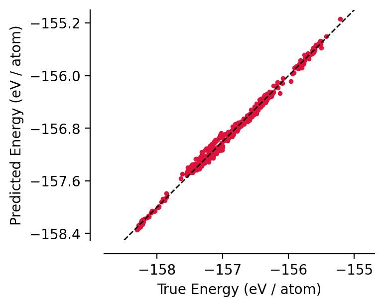
We can see from a single data point that our model has done a reasonable job of learning the PES:
[6]:
calculator.get_potential_energy(test[0]), test[0].info["energy"]
[6]:
(-9994.06640625, np.float64(-9998.70784))
graph-pes provides a few utility functions for visualising model performance:
[7]:
import matplotlib.pyplot as plt
from graph_pes.utils.analysis import parity_plot

%config InlineBackend.figure_format = 'retina'

parity_plot(
    best_model,
    test,
    property="energy_per_atom",
    units="eV / atom",
    lw=0,
    s=12,
    color="crimson",
)
plt.xlim(-158.5, -155)
plt.ylim(-158.5, -155);
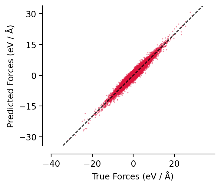
[8]:
parity_plot(
    best_model,
    test,
    property="forces",
    units="eV / Å",
    lw=0,
    s=2,
    alpha=0.5,
    color="crimson",
)
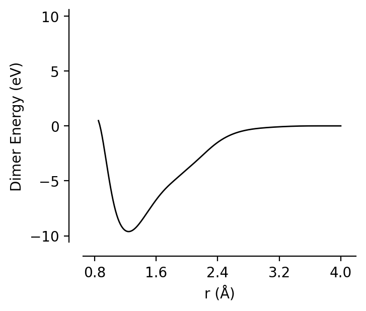
[9]:
from graph_pes.utils.analysis import dimer_curve

dimer_curve(best_model, system="CC", units="eV", rmin=0.85, rmax=4.0);
Beyond static evaluations, there are many more use cases for these models - head over to e.g. our ASE examples notebook for more details