Implement a model
FYI, you can open this notebook in Google Colab and follow along interactively 😊
Any and all GraphPESModel subclasses are fully compatible with graph-pes! You can:
train them using
graph-pes-trainrun MD in LAMMPS using
pair_style graph_pesload and analyse them using load_model
To demonstrate this, below we’ll implement a somewhat arbitrary model, and train it on the QM7 dataset.
Implementation
This model generates embeddings of neighbouring atoms as a function of their distance from the central atom and their atomic number.
These embeddings are summed over all neighbouring atoms to generate an embedding of the local environment, before being read out to predict the local energy:
[3]:
%%writefile custom_model.py

from __future__ import annotations

import torch
from graph_pes import AtomicGraph, GraphPESModel
from graph_pes.atomic_graph import (
    PropertyKey,
    index_over_neighbours,
    neighbour_distances,
    sum_over_neighbours,
)
from graph_pes.models.components.distances import Bessel, PolynomialEnvelope
from graph_pes.utils.nn import MLP, PerElementEmbedding


class CustomModel(GraphPESModel):
    def __init__(
        self,
        cutoff: float,
        channels: int,
        radial_features: int,
    ):
        super().__init__(
            cutoff,
            implemented_properties=["local_energies"],
        )

        # node embeddings
        self.Z_embedding = PerElementEmbedding(channels)

        # messages
        self.radial_basis = Bessel(radial_features, cutoff)
        self.envelope = PolynomialEnvelope(cutoff)
        self.message = MLP(
            layers=[
                radial_features + channels,
                2 * channels,
                2 * channels,
                channels,
            ],
            activation="CELU",
            bias=False,
        )

        # readout
        self.readout = MLP(
            layers=[channels, channels, 1],
            activation="CELU",
        )

    def forward(self, graph: AtomicGraph) -> dict[PropertyKey, torch.Tensor]:
        # compute the local energies
        # assume that the input graph has N atoms, E edges
        # and denote the number of radial features as R
        # and the number of channels as C

        # 1. embed node features
        h = self.Z_embedding(graph.Z)  # (N, C)

        # 2. expand distances
        r = neighbour_distances(graph)  # (E,)
        r_features = self.radial_basis(r)  # (E, R)
        r_features = self.envelope(r_features)  # (E, R)

        # 3. create neigbour embeddings
        h_neighbour = index_over_neighbours(h, graph)  # (E, C)
        neighbour_embeddings = torch.cat(
            [h_neighbour, r_features], dim=-1
        )  # (E, C + R)

        # 4. create messages
        messages = self.message(neighbour_embeddings)  # (E, C)

        # 5. aggregate messages
        aggregated_messages = sum_over_neighbours(messages, graph)  # (N, C)

        # 6. update node embeddings
        h = h + aggregated_messages  # (N, C)

        # 7. readout
        local_energies = self.readout(h).squeeze(-1)  # (N,)

        return {"local_energies": local_energies}
Writing custom_model.py
We can now use and instantiate our model as normal:
[4]:
from ase.build import molecule
from custom_model import CustomModel
from graph_pes import AtomicGraph

model = CustomModel(cutoff=5.0, channels=3, radial_features=8)
graph = AtomicGraph.from_ase(molecule("H2O"))
model(graph)
[4]:
{'local_energies': tensor([0.6992, 0.4318, 0.4318], grad_fn=<SqueezeBackward1>)}
We get all the functionality of a GraphPESModel for free:
[5]:
model.get_all_PES_predictions(graph)
[5]:
{'energy': tensor(1.5627, grad_fn=<SumBackward1>),
 'forces': tensor([[-0.0000e+00, -0.0000e+00, -1.2980e-05],
         [-0.0000e+00, -7.9464e-06,  6.4898e-06],
         [-0.0000e+00,  7.9464e-06,  6.4898e-06]], grad_fn=<NegBackward0>),
 'local_energies': tensor([0.6992, 0.4318, 0.4318], grad_fn=<SqueezeBackward1>)}
Training
Let’s train our architecture on the QM7 dataset. Below, we use load-atoms to load this dataset, and save the training and validation, splits to files train.xyz and val.xyz:
[6]:
from ase.io import write
from load_atoms import load_dataset

dataset = load_dataset("QM7")
train, val, test = dataset.random_split([1000, 100, 500])
write("train.xyz", train)
write("val.xyz", val)
Our configuration file is as normal (see the graph-pes-train guide for more details):
[7]:
%%writefile config.yaml

model:
    +custom_model.CustomModel:
        cutoff: 5.0
        channels: 3
        radial_features: 8

data:
    train: train.xyz
    valid: val.xyz

loss: +PerAtomEnergyLoss()

fitting:
    trainer_kwargs:
        max_epochs: 150
        accelerator: cpu
        check_val_every_n_epoch: 5

    optimizer:
        name: AdamW
        lr: 0.001

    loader_kwargs:
        batch_size: 64

general:
    run_id: custom-model-run
    progress: logged

wandb: null
Writing config.yaml
[8]:
!graph-pes-train config.yaml
[graph-pes INFO]: Started `graph-pes-train` at 2024-12-05 15:23:22.097
[graph-pes INFO]: Successfully parsed config.
[graph-pes INFO]: ID for this training run: custom-model-run
[graph-pes INFO]:
Output for this training run can be found at:
   └─ graph-pes-results/custom-model-run
      ├─ logs/rank-0.log    # find a verbose log here
      ├─ model.pt           # the best model
      ├─ lammps_model.pt    # the best model deployed to LAMMPS
      └─ train-config.yaml  # the complete config used for this run

GPU available: True (mps), used: False
TPU available: False, using: 0 TPU cores
HPU available: False, using: 0 HPUs
[graph-pes INFO]: Logging to graph-pes-results/custom-model-run/logs/rank-0.log
[graph-pes INFO]: Preparing data
[graph-pes INFO]: Setting up datasets
[graph-pes INFO]: Pre-fitting the model on 1,000 samples
[graph-pes INFO]: Number of learnable params : 159
[graph-pes INFO]: Sanity checking the model...
[graph-pes INFO]: Starting fit...
                            valid/metrics   valid/metrics   timer/its_per_s   timer/its_per_s
   epoch      time   per_atom_energy_rmse     energy_rmse             train             valid
       5       0.9                0.95875        15.93489         142.85715         225.00000
      10       1.9                0.86565        12.73514         125.00000         250.00000
      15       2.8                0.83548        12.34085         142.85715         225.00000
      20       3.8                0.80516        11.67857         142.85715         225.00000
      25       4.7                0.75636        11.28497         142.85715         250.00000
      30       5.6                0.67931         9.89885         142.85715         266.66669
      35       6.6                0.47443         6.82189         125.00000         225.00000
      40       7.6                0.30103         4.54500         125.00000         225.00000
      45       8.6                0.29590         4.52308          90.90909         183.33334
      50       9.6                0.30439         4.76209         111.11111         250.00000
      55      10.5                0.28471         4.38400         142.85715         225.00000
      60      11.7                0.28413         4.37031         125.00000         200.00000
      65      12.6                0.27077         4.18555         142.85715         266.66669
      70      13.5                0.26347         4.06702         142.85715         225.00000
      75      14.5                0.25786         3.99087         111.11111         225.00000
      80      15.4                0.25494         3.93345         142.85715         250.00000
      85      16.4                0.24410         3.77900         125.00000         225.00000
      90      17.3                0.23976         3.70559         125.00000         208.33334
      95      18.3                0.23695         3.71650         142.85715         225.00000
     100      19.2                0.23006         3.61704         142.85715         225.00000
     105      20.2                0.21487         3.33465         125.00000         225.00000
     110      21.1                0.20718         3.20724         166.66667         225.00000
     115      22.1                0.20142         3.11764         125.00000         225.00000
     120      23.1                0.18958         2.94265         142.85715         250.00000
     125      24.0                0.18257         2.83350         142.85715         291.66669
     130      25.1                0.17456         2.71116         142.85715         225.00000
     135      26.3                0.16515         2.58272         125.00000         225.00000
     140      27.2                0.16033         2.48846         142.85715         250.00000
     145      28.2                0.15938         2.47974         111.11111         208.33334
     150      29.2                0.14885         2.31319         142.85715         225.00000
`Trainer.fit` stopped: `max_epochs=150` reached.
[graph-pes INFO]: Loading best weights from "graph-pes-results/custom-model-run/checkpoints/best.ckpt"
[graph-pes INFO]: Training complete. Awaiting final Lightning and W&B shutdown...
Analysis
We can now load our trained model and analyse the results:
[9]:
from graph_pes.models import load_model

model = load_model("graph-pes-results/custom-model-run/model.pt")
model
[9]:
CustomModel(
  (Z_embedding): PerElementEmbedding(dim=3, elements=[])
  (radial_basis): Bessel(n_features=8, cutoff=5.0, trainable=True)
  (envelope): PolynomialEnvelope(cutoff=5.0, p=6)
  (message): MLP(11 → 6 → 6 → 3, activation=CELU(alpha=1.0))
  (readout): MLP(3 → 3 → 1, activation=CELU(alpha=1.0))
)
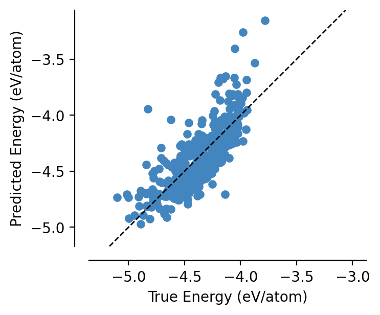
This is a very unsophisticated architecture, so we don’t expect it to be particularly accurate…
[10]:
from graph_pes.utils.analysis import parity_plot

%config InlineBackend.figure_format = 'retina'

parity_plot(
    model,
    test,
    property="energy_per_atom",
    units="eV/atom",
)
MD
Running MD with our new model architecture is straightforward.
Below, we use ASE-driven MD for simplicity - please see the LAMMPS MD guide for instructions on how to run MD with our model in LAMMPS.
[18]:
from ase import units
from ase.build import molecule
from ase.md.langevin import Langevin

# set up calculator and structure
calculator = model.ase_calculator()
structure = molecule("CH4")
structure.center(vacuum=3.0)  # place in a large unit cell
structure.pbc = True

# set up MD
structure.calc = calculator
dynamics = Langevin(
    structure,
    timestep=0.1 * units.fs,
    temperature_K=300,
    friction=0.01 / units.fs,
)
dynamics.attach(
    lambda: structure.write("dump.xyz", append=True),
    interval=100,
)

# run MD
dynamics.run(1000)  # 1000 steps = 0.1 ps
[18]:
True
Unsurprisingly, our very simple model has not been able to keep the simulation stable:
[19]:
from load_atoms import view

view(structure, show_bonds=True)
[19]: